
What Is Search Clustering? A Simple Guide to How It Groups Related Results

TL;DR
You open a document set or search results page and immediately hit the same problem: forty results, no clear grouping, and three minutes wasted scanning before you find what you actually needed.
Most people assume sorting by relevance score solves this. It does not. A flat ranked list treats every item as independent. Two results about the same concept land six rows apart, and a reader scanning quickly misses one or both.
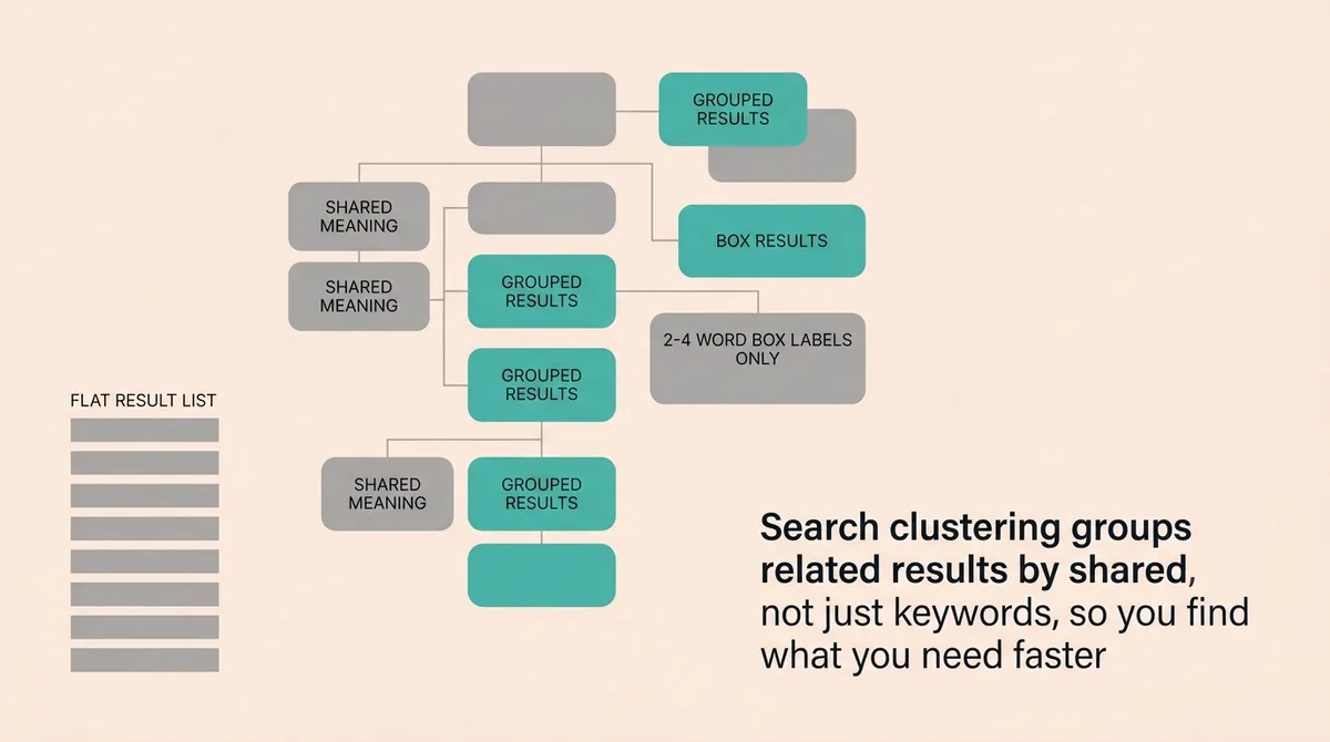
Search clustering is the mechanism that pulls related results toward each other based on shared meaning, not surface word overlap. The grouping logic measures semantic distance between items, then separates distinct topics into distinct clusters. Content leads managing large document libraries and SEO agency founders auditing keyword sets both benefit from understanding how grouping decisions get made, and where they silently break down.
What is search clustering and how does it group related results?
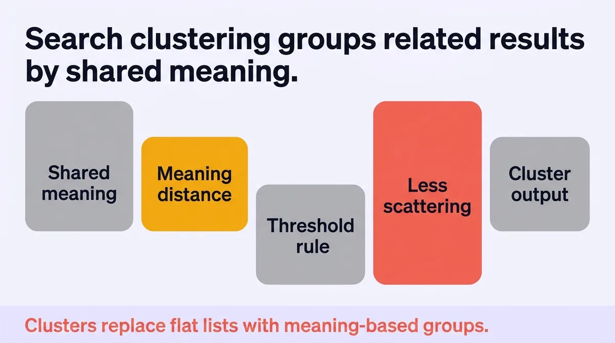
Search clustering is a method of organizing results by shared meaning or intent, so that items covering the same idea appear together rather than scattered. The grouping logic calculates how close two results are in meaning, then assigns them to the same cluster when that distance falls below a set threshold. The output is a structured set of groups rather than a single flat list.
What Search Clustering Actually Does and Why the Basic Definition Misses the Point
Most definitions describe search clustering as “grouping similar results.” That framing is technically accurate and practically useless.
Grouping by similarity could mean grouping by file type, by date, by author, or by shared words. None of those approaches produce what clustering actually produces. The real mechanism groups by shared meaning, and meaning is not the same as shared vocabulary.
Two documents can use completely different words and still belong in the same cluster. Two documents can share ten keywords and belong in completely different clusters. The distinction matters because it changes what gets surfaced and, more importantly, what gets buried.
Here is the sting line: clustering is not a labeling system. It is a decision about what the system treats as the same idea.
A practical implementation of this is entity mapping, where relevance scores sit on a 0 to 1 scale [2]. A result mapped to an entity at 0.9 relevance belongs in a different cluster position than a result mapped at 0.3, even if both contain the same keyword. The score reflects meaning proximity, not word frequency.
Mapping may be limited to roughly 5 entities per search item [2]. That cap forces the system to commit. It cannot treat a result as equally relevant to ten different topics. It has to decide where the item belongs, which is exactly what clustering requires.
Stop thinking of this as a cosmetic layer on top of search results. It is the layer that decides which ideas your reader sees grouped as equivalent and which ideas get treated as distinct.
How the Grouping Logic Decides What Belongs Together and What Gets Separated
The grouping decision starts with a measurement. Every result gets compared to every other result. The comparison produces a distance value. Small distance means close in meaning. Large distance means far apart.
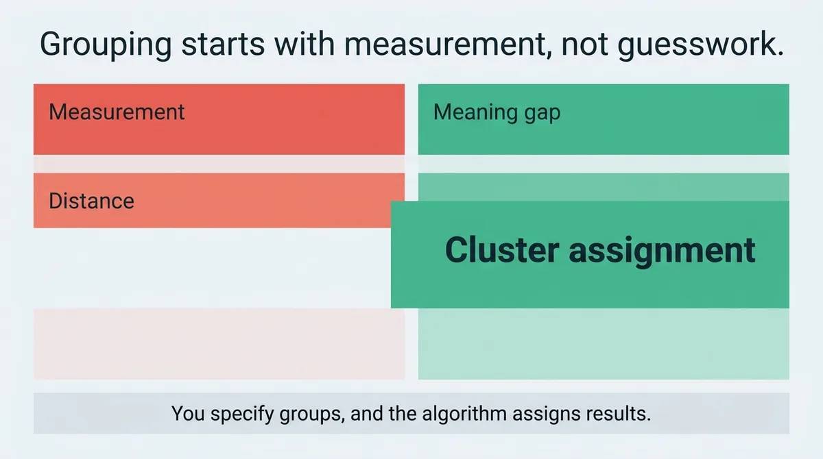
What happens next depends on the algorithm. K-means, one of the most common approaches, requires you to specify the number of clusters in advance [1]. You tell the system: “I want five groups.” The algorithm then assigns every result to whichever of those five groups it fits best.
The practical consequence of that requirement is often invisible to people who read about clustering casually. If you specify five groups but the data naturally forms three meaningful clusters and two noise groups, the algorithm still produces five. Two of those groups will be artificial splits of real clusters. The reader sees six results where they expected coherence, and finds mild confusion instead.
Running K-means multiple times with different starting configurations reduces that risk [1]. Each run produces a slightly different grouping. The system picks the run that produces the tightest clusters. Tighter clusters mean items inside a group are closer to each other in meaning.
Affinity propagation takes a different path. It does not require you to specify a number of clusters. Items vote for which other item best represents them, and the algorithm finds natural group centers. The cost is computational. Affinity propagation scales at roughly O(N²T) in time and O(N²) in memory when using a dense similarity matrix [1]. For large result sets, that cost becomes prohibitive quickly.
That is why affinity propagation is most appropriate for small to medium-sized datasets [1]. A library of 200 internal documents is a reasonable use case. A search index of two million documents is not.
The friend advice version of this: stop picking a clustering algorithm based on what sounds most sophisticated. Pick based on how many items you are grouping. Wrong algorithm choice is one of the most common reasons clustering outputs look reasonable but feel wrong to actual users.
Two distinct clustering paths appear in documented implementations: one uses ontology-based merging after first-level clusters form, and another combines ontology with an embedding space [2]. The ontology path groups by known conceptual relationships. The embedding path groups by learned semantic proximity. Each produces a different cluster shape for the same input data.
Approach | Input Required | Best Fit |
|---|---|---|
K-means | Number of clusters specified | Large structured datasets |
Affinity propagation | Similarity matrix | Small to medium datasets |
Ontology-based merging | Defined concept hierarchy | Domain-specific knowledge bases |
The table above shows three distinct paths. Each one changes which items end up together and which get separated. The choice is not neutral.
The Hidden Cost of Skipping Clustering: Why Flat Result Lists Quietly Destroy Usability
A flat list feels clean. One column, ranked by score, top to bottom. The problem is not visible until a user starts scanning.
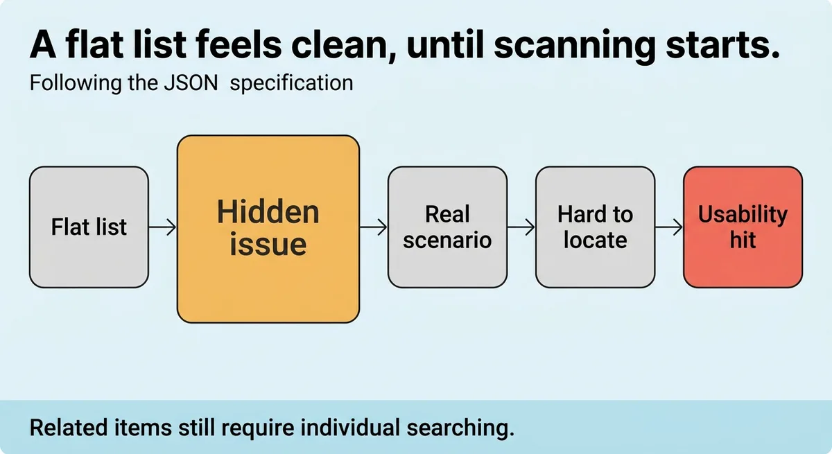
Imagine a content lead at a B2B SaaS company opening a 60-result export from their content audit tool. They need to find all articles related to onboarding workflows. Without clustering, those articles might sit at positions 3, 17, 31, and 44 in the ranked list. Each one has to be found individually. Three minutes of scanning becomes fifteen. Multiply that by a team of four doing weekly audits, and the time loss is measurable.
That is not an abstract inefficiency. That is a direct cost to review cycles and editorial capacity.
Affinity propagation’s O(N²) memory scaling [1] illustrates the flip side. Systems that try to cluster large sets without accounting for scale collapse under their own computational weight. The result is either a crash, a timeout, or a silently degraded output where items that should cluster together get dropped from the grouping entirely. The user sees a smaller result set and assumes the information does not exist.
The patent literature on entity-based clustering describes two paths for merging first-level clusters [2]. One uses ontology alone. One combines ontology with an embedding space. Systems that skip both paths and rely only on keyword frequency produce clusters that look correct but break on edge cases. A document about “account recovery” and a document about “password reset” belong in the same cluster for most user intents. Keyword-only grouping often separates them because the word overlap is low.
The directional signal here: every time a user queries a result set and reformulates their query without changing what they actually want, that is a clustering failure. They are compensating for the system’s inability to group what they need. That reformulation behavior is a measurable proxy for how often flat lists force users to do the system’s job manually.
What Good Clustering Looks Like in Practice and What Most Guides Get Wrong About It
Most guides describe good clustering as “tight” and “well-separated.” Both terms are accurate. Neither tells you what to actually look for when evaluating results.
A well-clustered result set has three visible properties. First, items inside a cluster share a specific idea, not just a general topic. “Project management software” and “project management for remote teams” belong in the same cluster. “Project management software” and “management consulting” do not, even though both contain the word “management.” Second, moving between clusters feels like a topic change, not a subtle variation. Third, every cluster contains enough items to be useful but not so many that it becomes its own flat list problem.
Mini-batch K-means draws samples in batches per training iteration [1]. That approach reduces computation time significantly on large datasets. The tradeoff is slightly less precise cluster assignments. For a content library with five thousand documents, slightly imprecise clusters that load in two seconds are more useful than perfect clusters that take forty seconds to generate.
That is a real implementation caveat most guides skip entirely. Precision and speed operate in tension. Choosing the wrong tradeoff produces clusters that are either too slow to be practical or too loose to be meaningful.
Certain methods accept similarity matrices rather than raw feature matrices [1]. Affinity propagation, spectral clustering, and DBSCAN can take a matrix of shape (n_samples, n_samples) rather than (n_samples, n_features) [1]. That distinction matters when you already have a computed similarity score between items and do not want to reprocess raw content. Plugging in the similarity matrix directly preserves relationships that raw feature extraction might flatten.
A real-world scenario: a three-person content agency ran manual keyword clustering for a client’s blog. They grouped 200 posts by hand, took four hours, and found seven thematic clusters. They then ran the same posts through a mini-batch approach with a similarity matrix input. The output matched five of the seven manual clusters exactly, split one cluster more accurately, and flagged one manual cluster as a false group. Total compute time: ninety seconds. The one false manual cluster had caused two months of content gaps in a topic area the client thought was covered.
Manual grouping created a blind spot. Matrix-based clustering removed it. The gap closed in the next content cycle.
Poor clustering output usually shows one of two failure signatures. Either clusters are too broad, meaning they contain items that feel loosely related but do not actually answer the same question, or clusters are too narrow, meaning each cluster contains two items and the grouping adds no navigation value. Both failures are correctable. Broad clusters usually mean the distance threshold is too loose. Narrow clusters usually mean the threshold is too tight or the number of clusters was set too high.
Why Grouping by Meaning Beats Grouping by Keyword Every Time
Keyword grouping is fragile. It breaks on synonyms. It breaks on phrasing variation. It treats “email deliverability” and “inbox placement rate” as different topics when most readers treat them as the same concern.
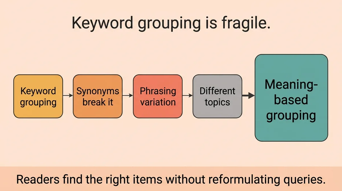
Meaning-based grouping captures intent. The system does not look for matching strings. It looks for matching conceptual territory. That shift changes what shows up together and, critically, what a reader finds without having to reformulate their query.
The two-path clustering framework described in entity-based implementations [2] reflects this directly. Ontology-based merging groups items by known conceptual relationships. Embedding-based grouping adds learned proximity from actual usage patterns. Combined, they produce clusters that hold up across phrasing variation.
For a content lead managing a stalled blog backlog, this means fewer lost articles and fewer gaps that only show up when someone audits the archive six months later. For an agency founder managing multiple client content libraries, it means cluster assignments that stay stable as new content gets added, rather than collapsing every time the keyword strategy shifts.
Grouping by keyword is a rule. Grouping by meaning is a decision about what belongs together. The two-path framework is where that decision gets made with precision.
References and Citations
[1]https://scikit-learn.org/stable/modules/clustering.html
[2]https://gofishdigital.com/blog/entity-clustering/
FAQ
Search clustering is a method of organizing results by shared meaning or intent, so that items covering the same idea appear together rather than scattered across a flat ranked list. The grouping logic calculates semantic distance between items and assigns them to the same cluster when that distance falls below a set threshold, producing structured groups instead of a single ranked column. This matters in practice because two documents can share zero keywords and still belong in the same cluster, while two documents that repeat the same keyword can belong in completely different ones. Platforms like Zelitho apply this logic at the topic-selection stage, so content plans are built around meaningful clusters rather than individual keyword matches.
Keyword grouping treats shared word strings as proof of shared topic, while semantic clustering groups by shared intent and conceptual proximity regardless of exact word overlap. Keyword grouping breaks on synonyms and phrasing variation, so terms like ’email deliverability’ and ‘inbox placement rate’ land in separate buckets even though readers treat them as the same concern. Semantic clustering uses either ontology-based merging, embedding-based proximity, or a combination of both to hold clusters stable across phrasing variation. The practical result is fewer content gaps and fewer articles that only surface in audits six months after they should have been found.
Use K-means when you have a large structured dataset and can specify the number of clusters in advance; use affinity propagation when you have a small to medium dataset and want the algorithm to find natural group centers without a preset count. K-means is faster and scales well, but it forces the number of groups you define even when the data supports fewer natural divisions, which can produce artificial splits that confuse readers. Affinity propagation scales at roughly O(N squared) in memory, making it prohibitively expensive on large indexes but well-suited to libraries of a few hundred documents. Mini-batch K-means is a practical middle path for large content libraries, trading a small amount of cluster precision for dramatically faster compute time.
Poor search clustering forces users to scan flat ranked lists manually, scattering related content across positions that require multiple reformulated queries to locate, which turns three-minute reviews into fifteen-minute ones and compounds across team size and audit frequency. A content team auditing 60 results without clustering might find related articles at positions 3, 17, 31, and 44, each requiring individual discovery. Every query reformulation that does not change what the user actually wants is a measurable clustering failure: the user is doing the system’s job by hand. Zelitho addresses this upstream by structuring topic selection around semantic clusters, so content gaps and duplicate coverage are visible before drafting begins rather than discovered in a post-publication audit.
A small content team can use search clustering to group existing posts by semantic proximity, which surfaces topic areas with dense coverage and others with genuine gaps that manual review often misses. Running a similarity-matrix-based clustering approach on even 200 posts takes under two minutes by machine, compared to four or more hours of manual grouping, and it can flag false clusters where content looks thematically grouped but does not actually answer the same reader question. One documented case showed a manually grouped false cluster that had hidden a two-month content gap in a topic area the team believed was fully covered. Zelitho builds clustered topic selection directly into its planning workflow, so teams see semantic groupings before they commission new articles rather than discovering coverage problems after publishing.